boxplot & bwplot

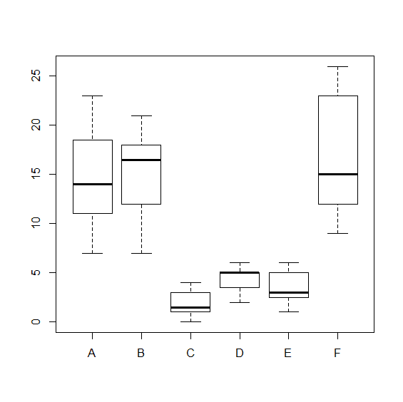
'boxplot' is perhaps thought of as another way of representing 'densityplot' or distribution of the data. Hence, it is useful for comparing data by groups or categories within the data.

It works well with large dataset, compared to scatter plots which struggles when there are too many data points to plot.

The graphic parameters used for boxplot() are similar to plot().

Example:

boxplot(count~spray,InsectSprays)

The above example show outliers. To remove these outliers from the graph, set 'outline' to FALSE.

boxplot(count~spray,InsectSprays,outline=FALSE)

'bwplot' is 'lattice' package's version of boxplot, and the graphic parameters used for boxplot() are similar to xyplot().

Example:


bwplot(uptake~Type,CO2)

To remove outliers, set do.out=FALSE.

bwplot(uptake~Type,CO2,do.out=FALSE)

With split panels,

bwplot(uptake~Treatment|Type,CO2)

To change colour of the median point

bwplot(uptake~Treatment|Type,CO2,col="red")

To change colour of the median point and rectangle frame,

bwplot(uptake~Treatment|Type,CO2,col="red",

par.settings=list(box.rectangle=list(col="salmon",alpha=0.4)))

To change colour of the median point, rectangle frame and rectangle body,

bwplot(uptake~Treatment|Type,CO2,col="red",

par.settings=list(box.rectangle=list(col="salmon",fill="salmon",alpha=0.4)))

To change colour of the median point, rectangle frame, rectangle body and umbrella,

bwplot(uptake~Treatment|Type,CO2,col="red",

par.settings=list(box.rectangle=list(col="salmon",fill="salmon",alpha=0.4),box.umbrella=list(col="salmon",alpha=0.4)))

To change colour of the median point, rectangle frame, rectangle body, umbrella and outlier,

bwplot(uptake~Treatment|Type,CO2,col="red",

par.settings=list(box.rectangle=list(col="salmon",fill="salmon",alpha=0.4),box.umbrella=list(col="salmon",alpha=0.4),plot.symbol=list(col="salmon",alpha=0.4)))

To overlap two bwplots for comparison,

bwplot(Sepal.Length~Species,iris,col="red",scale=list(y=list(lim=c(0,10))),key=list(space="top",column=2,text=list(label=c("Sepal Length","Petal Length"),cex=0.8,col="darkgrey"),

rectangles=list(col=c("salmon","dodgerblue"),rectangles=c("salmon","dodgerblue"),alpha=0.4,size=3)),

par.settings=list(box.rectangle=list(col="salmon",fill="salmon",alpha=0.4),box.umbrella=list(col="salmon",alpha=0.4),plot.symbol=list(col="salmon",alpha=0.4)))+

as.layer(bwplot(Petal.Length~Species,iris,col="blue",

par.settings=list(box.rectangle=list(col="dodgerblue",fill="dodgerblue",alpha=0.4),box.umbrella=list(col="dodgerblue",alpha=0.4),plot.symbol=list(col="dodgerblue",alpha=0.4)))

)

Blank Plots & Graphic Devices

To create blank plots, there are few options:

from 'base' package:

plot.new()

frame()

plot(1,type="n",axes=FALSE,xlab="",ylab="")

blank plots without margins

par(mar=rep(0,4)) 

plot(1,type="n",axes=FALSE,xlab="",ylab="")

using 'lattice' package:

xyplot(1~1,col="transparent",scales=list(draw=FALSE),xlab="",ylab="",par.settings=list(axis.line=list(col=0)))

To open graphic device:

x11()       #for linux, but also works for other OS if installed  

windows()     #for windows  

quartz()      #for Mac 

Regular Expression

Regular expression can be used in R to substitute, extract or search of pattern of texts.


To extract a part of texts, we can use sub() with "\\n" as the replacement (n is an integer, usually 1 or 2). The example extracts date from a file name "ABC_2014_10_23.csv".

sub("^[A-Za-z]+(_)([0-9]{4}(_)[0-9]{2}(_)[0-9]{2})(.)[A-Za-z]+","\\2","ABC_2014_10_23.csv")

"2014_10_23"


To replace certain words with another| word, we can do the following.

gsub("\\s*\\b(meters|m|meter)\\b","m",
"DAS FE TDAS 5meter ADSA RE 12 meters SA 23 Meters DASD 3 m",
ignore.case=TRUE)

"DAS FE TDAS 5meter ADSA RE 12m SA 23m DASD 3m"


To find fields matching the pattern, we can use grep().

The below looks for numbers followed by alphabet:

A<-c("SDA09DA","ADCZFD","081382","ASDF8673")
A[grep("[A-Z]+[0-9]+",A)]

"SDA09DA"  "ASDF8673"


The below looks for numbers between alphabets:

A<-c("SDA09DA","ADCZFD","081382","ASDF8673")
A[grep("[A-Z]+[0-9]+[A-Z]",A)]

"SDA09DA"


The below looks for more complex pattern. This example looks for typical address format.

A<-c("100 ASD ST DASER","CSADAS SS ASD ADA",
"321 DSA XCSACXZ SADAS 213","321/32 ASA ASDDD RD WEASF",
"DSA 231 DDG BGBVCVB","SUITE 1/43 SAFDSA AVE ASDA",
"UNIT 21/2 ADSD AV SDADFF")

A[grep("^[A-Z]*\\s*[0-9]+\\s*(/)*\\s*[0-9]*\\s*[A-Z]+\\s*[A-Z]*\\s*(ST|RD|AVE|AV)\\s*[A-Z]*$",A)]

"100 ASD ST DASER"           
"321/32 ASA ASDDD RD WEASF" 
"SUITE 1/43 SAFDSA AVE ASDA" 
"UNIT 21/2 ADSD AV SDADFF"  



For more regular expression language, go to either of the following websites:

http://msdn.microsoft.com/en-us/library/az24scfc(v=vs.110).aspx

http://www.rexegg.com/regex-quickstart.html

Functions for Arithmatic

The following are some of the useful functions of arithmatic in R apart from +, -, *, /, ^ and sqrt()


To set limits before using scientific notation for large numbers, you can set the 'scipen' parameter within options(). The default limit is 10^12 for displaying in R console and 10^7 for the graphic device.

The below is larger than 10^13, and R reverts to using scientific notation.

31423190532586

3.142319e+13


By setting the option to scipen=15, the same number is retained in its natural form.

options(scipen=15)
31423190532586

31423190532586


For plotting:

plot(1:10,seq(0,100000000,length=10))

 

options(scipen=8)
plot(1:10,seq(0,100000000,length=10))




















To round the figure to significant figures, you can use the below function.

signif(12645.654,digits=2)

13000


signif(0.00034526,digits=2)

0.00035



For rounding figures, you can do the following.

round(12645.654)  #rounds to integer

12646


round(12645.654,digits=2) #rounds to second decimal place

12645.65


round(0.00034526,digits=5)

0.00035



To find ceiling (smallest integer large than the given number) of a figure, you can do the following.

ceiling(12645.654)  

12646


ceiling(0.00034526)  

1


To find ceiling (largest integer smaller than the given number) of a figure, you can do the following.

floor(12645.654)

12645


floor(0.00034526)  

0



To find absolute figure, you can do the following.

abs(-243)

243


To find the remainder of a division, you can use '%%', but this does not work well with large numbers

15%%2

1


To find quotient of a division (integer part of division output), you can use '%/%'.

15%/%2

7

arranging layout of lattice graphs using gridExtra package

gridExtra allows arranging multiple graphs in the device, even when those graphs are drawn from different data sources. This package only work for lattice and ggplot graphs.


library(lattice)
library(grid)
library(gridExtra)

dat<-aggregate(peri~perm,rock,sum)

dat1<-aggregate(rock[,c("peri","shape")],by=list(rock$perm),sum)
colnames(dat1)[1]<-"perm"


p1<-barchart(peri~factor(perm),dat,xlab="perm",ylab="peri",
main="data: rock aggregated 1",horizontal=FALSE,col="coral2",border="coral2")

p2<-xyplot(shape~factor(perm),dat1,xlab="perm",ylab="shape",col="seagreen2",
type="l",lty=1,lwd=2,main="data: rock aggregated 2")

p3<-xyplot(shape~peri,rock,xlab="peri",ylab="shape",col="maroon2",type="p",
cex=1.5,main="data: rock",pch=16)



grid.arrange(p1,p2,p3,ncol=1)





























grid.arrange(p2,arrangeGrob(p1,p3,widths=c(3/5,2/5),ncol=2),ncol=1)

To add the header or title,


grid.arrange(p2,arrangeGrob(p1,p3,widths=c(3/5,2/5),ncol=2),ncol=1,
main=textGrob("Rock",gp=gpar(cex=1.5,col="red")))


gridExtra versions later than 2.0.0 need to use "top" instead of "main" and "bottom" instead of "sub" for titles and subtitles respectively.


  

  
  
























To include a table in the display:


TBL<-summary(dat)

grid.arrange(arrangeGrob(
tableGrob(TBL, gp = gpar(cex = 0.8), show.rownames = FALSE, 
padding.h = unit(5, "mm")), 
p2, ncol = 2, widths = c(2/5, 3/5)), 
arrangeGrob(p1, p3, widths = c(3/5, 2/5), ncol = 2), ncol = 1,
main = textGrob("Rock", gp = gpar(cex = 1.5, col = "red")))



gridExtra versions later than 2.0.0 do not use gpar for tableGrob, hence the below code will need to be used instead.

  

grid.arrange(arrangeGrob(
tableGrob(TBL, theme = ttheme_default(core = list(fg_params = list(cex=0.8, hjust = 0.5)),
colhead = list(fg_params = list(cex=0.8))), rows = NULL), 
p2, ncol = 2, widths = c(2/5, 3/5)), 
arrangeGrob(p1, p3, widths = c(3/5, 2/5), ncol = 2), ncol = 1,
top = textGrob("Rock", gp = gpar(cex = 1.5, col = "red")))

The gridExtra version >= 2.0.0 allows more formatting options for tableGrob. For example, changing colours of background:

  

grid.arrange(arrangeGrob(
tableGrob(TBL, theme = ttheme_default(core = list(fg_params = list(cex=0.8, hjust = 0.5),
bg_params = list(fill = c("tan", "wheat"))),
colhead = list(fg_params = list(cex = 0.8, col = "white"), bg_params = list(fill = "brown"))), rows = NULL), 
p2, ncol = 2, widths = c(2/5, 3/5)), 
arrangeGrob(p1, p3, widths = c(3/5, 2/5), ncol = 2), ncol = 1, 
top = textGrob("Rock", gp = gpar(cex = 1.5, col = "red")))